Data wrangling

Welcome to Lab 3!

In our previous session we learned about R packages, including how to install and load them. We talked about the main types of data used in social science research and how to represent them in R. We also played around with some datasets using some key functions, such as: filter(), select(), and mutate(). In this session, we will build on these principles and learn how to import data in R, as well as clean and format the data using a real-world dataset. This is a common and important phase in quantitative research.

NoteOverview

By the end of this lab you will know how to:

• set up an RStudio project file from scratch
• create an R script to download, wrangle, and save a dataset
• load a saved dataset within an R Markdown file
• work with the dataset used in the formative and summative assessments

The NILT 2012 Dataset

Today, we will be working with data generated by the Access Research Knowledge (ARK) hub. ARK conducts a series of surveys about society and life in Northern Ireland. For this lab, we will be working with the results of the Northern Ireland Life and Times Survey (NILT) in the year 2012. In particular, we will be using a teaching dataset that focuses on community relations and political attitudes. This includes background information of the participants and their household.

NILT RStudio Project

We will continue using Posit Cloud, as we did in the previous labs. This time though we are going to make a new RStudio project from scratch.

Within your “Lab Group …” workspace in Posit Cloud (if you have not joined a shared space, follow the instructions in Lab 2) and:

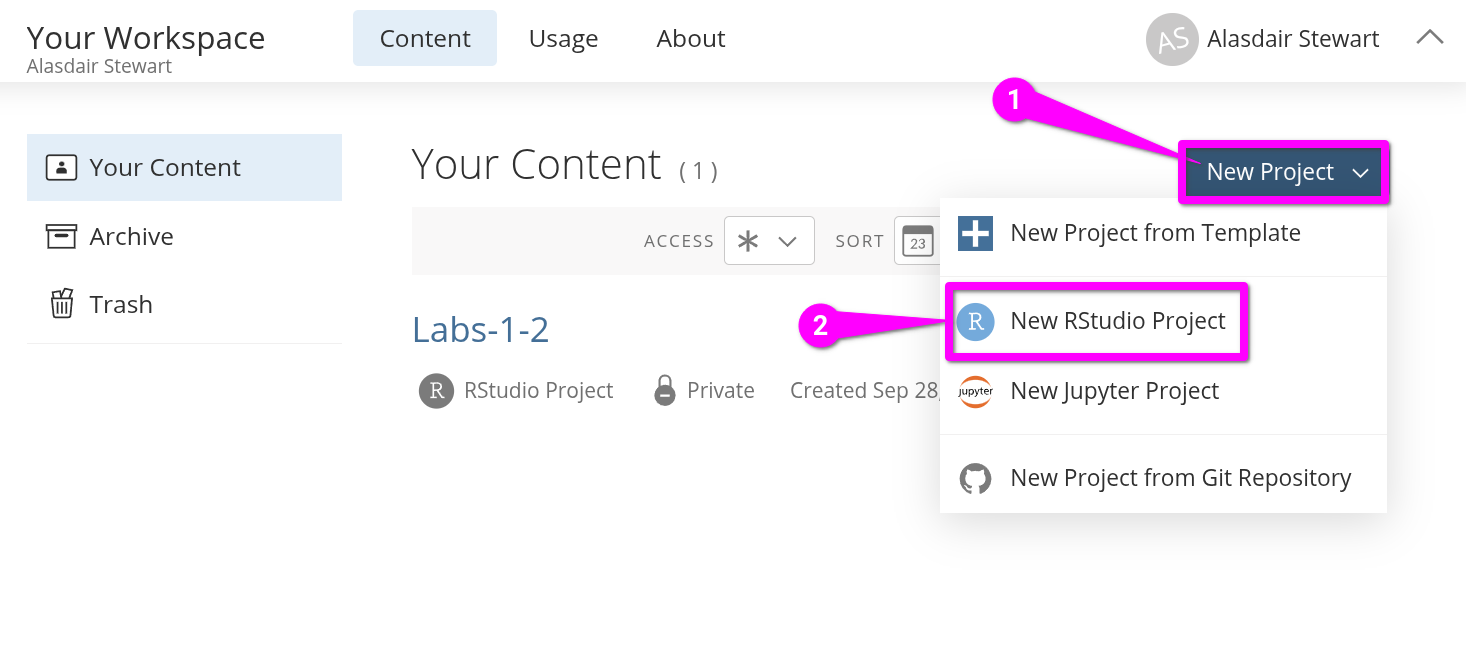
1. Click the blue ‘New Project’ button in the top-right.
2. From the list of options select ‘New RStudio Project’.

Once the project has loaded, click on ‘Untitled Project’ at the top of the screen.

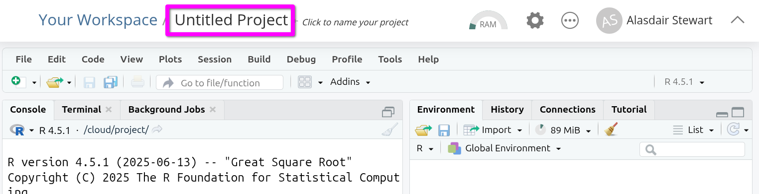
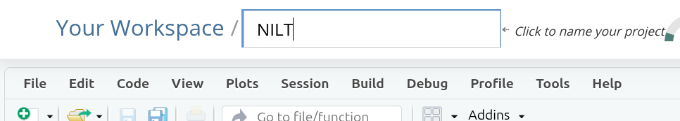
You can now give your project a name. This is how it will appear in your list of projects in your lab group workspace. Let’s name it “NILT” as we will use this project to work with the NILT data. Type the name and hit Enter to confirm.

Creating an R Script

Although this project is just for the labs, we are going to set it up in a ‘reproducible’ way. This means anyone with a copy of our project would be able to run the code and receive the same results as us. Last week, we downloaded a data set using the Console. This week we will instead cover one way to include the code used to download and wrangle our data in a file separate to the R Markdown files we use for the analysis.¹

(As you will see with the RStudio templates used for the assessments, it is possible to share an RStudio Project with the data. However, that is not always possible or desirable. For instance, the data whilst available for anyone to download from an organisation’s website or data archive may have license restrictions prohibiting making a version of it available elsewhere.)

To do this we will use an R script file. In our first two labs we used R Markdown, which lets us create code chunks for adding our R code. An R script file is simply a file that contains only R code, like a giant code chunk.

By convention, R scripts for doing set up, data prep, and similar are placed in an ‘R’ subfolder. To create one:

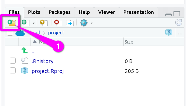
1. In the “Files” pane (bottom-right) click the folder icon that also has a green circle with white plus in it.

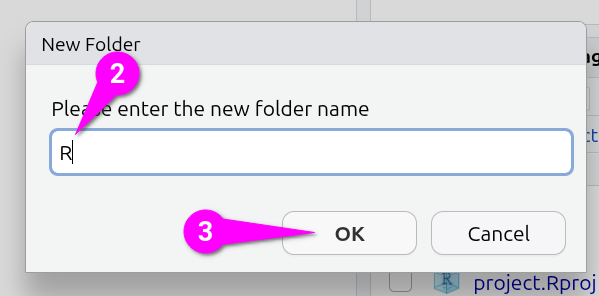
Then, within the ‘New Folder’ dialog that will pop up:

2. Type a single letter capital ‘R’ as the name.
3. Click the ‘OK’ button to confirm creation of the folder.

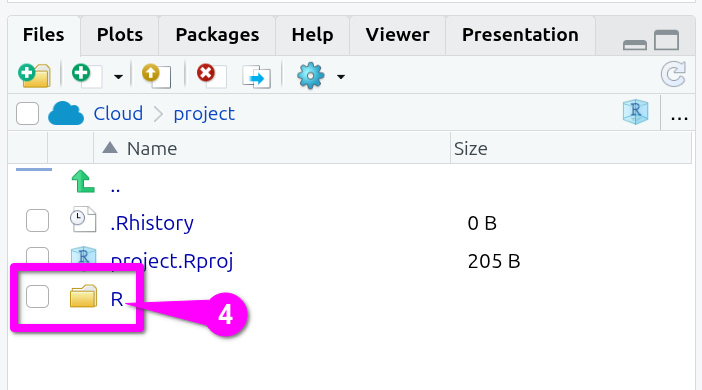
You should now see the new folder in the bottom-right panel, so -

4. Click the ‘R’ folder to navigate into it (Note, you need to click the ‘R’ and not the folder icon.)

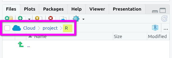
You should now see an empty folder, and can double-check you are in the right folder by looking at the navigation bar which should be “Cloud > project > R”.

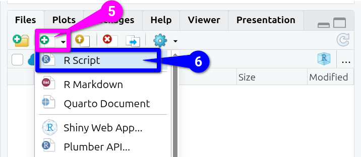
OK, now:

5. Click the white document icon that is to the right of the new folder icon you clicked before. (See screenshot below!)
6. From the list of options click ‘R Script’

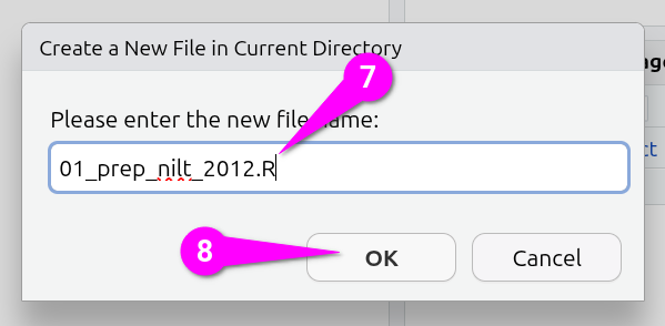
That will bring up a ‘Create a New File in Current Directory’ dialog:

7. Name your file 01_prep_nilt_2012.R
8. Click the ‘OK’ button to confirm creation of the script

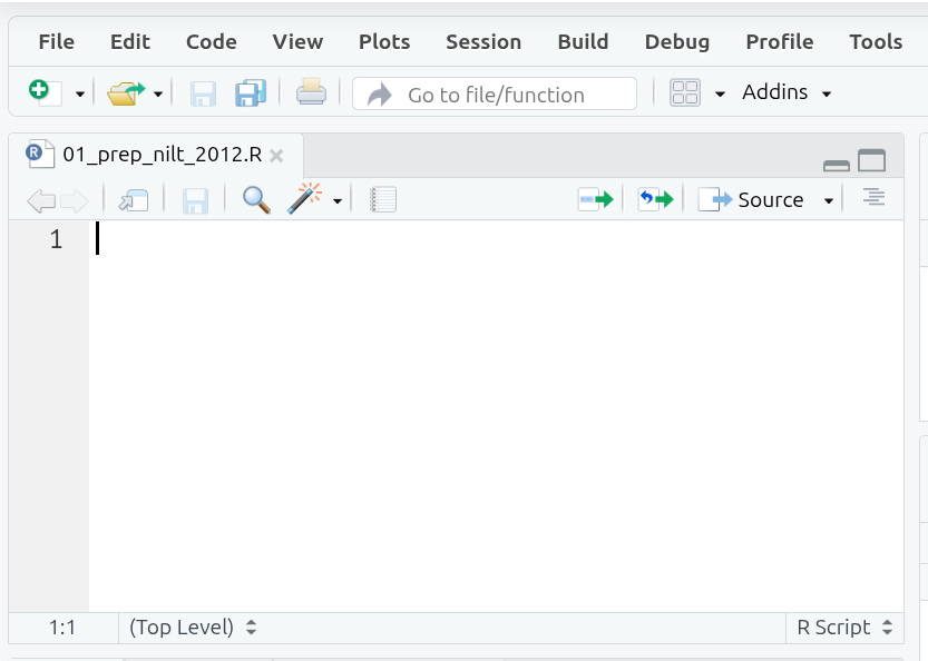
The file should then auto open in the top-left pane.

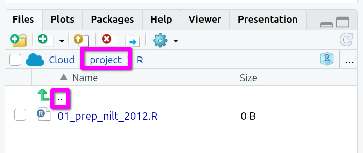
Lastly, before we move to writing our R script, let’s navigate back to the top-level folder of our project in the ‘Files’ pane (bottom-right). To navigate back up to the top-level folder, click either the ‘..’ at the top of the folder content list or in the navigation bar click the ‘project’ text.

Installing and Loading Packages

Back to our top-left pane with our R script. It is good practice to include some key information in this file, such as what it does, when it was written, and who wrote it. Given R script is all R code, we can add this info using comments. As a reminder, any line in R that begins with a ‘#’ is treated as a comment and will not be run as part of the code.

Below is a template you can use.

## Download and process NILT 2012 survey

# Date: [add today's date here]
# Author: [add your name here]

The ‘##’, with an extra ‘#’, at the top doesn’t do anything extra or different, we just include it to make visually clear this is the title / short description of what the script does.

Next, it is good practice to include details for the data set being used, especially important if the data is not our own to ensure proper attribution. In addition to being good practice, it is often a condition for data sets where it is permitted to re-share them elsewhere that you can do so only as long as you include an attribution (i.e. a reference).

Let’s then add a reference section. (Feel free to use the clipboard button in top-right of the box below to copy and paste the text.)

# References  -----------------------------------------------------------------

# https://www.ark.ac.uk/teaching/
# 2012 Good relations: ARK. Northern Ireland Life and Times Survey Teaching Dataset 2012, Good relations [computer file]. ARK www.ark.ac.uk/nilt [distributor], March 2014.

The ----- after # References again doesn’t do anything aside from help make the section visually distinct. This may seem odd at the moment, but as the file grows in length, the importance of making it easy to find sections quickly from visual glance starts to make sense.

OK, let’s now install packages that are needed for our project. Remember we need to do this every time we create a new project on Posit Cloud. If using RStudio Desktop, we would only need to install packages once per device we are using rather than per project.

However, compared to last week, we want to set up our project so that anyone can run the code and achieve the same results. (If we run into irrepairable errors we may also want to re-run our R scipt to ‘reset’ our project). We will not know though what packages someone will already have installed or not.

Thankfully, we can write R code in our script that will check whether specific packages are already installed, and then install any packages needed that are missing.

First, add a comment to make clear there is a new section:

# Packages -------------------------------------------------------------------

Next, add the following comment and code:

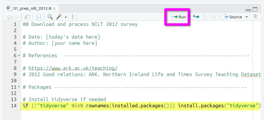
# Install tidyverse if needed
if (!"tidyverse" %in% rownames(installed.packages())) install.packages("tidyverse")

This code may look complex, but it is largely the number of brackets making it looks more complex than it actually is:

• if checks whether a given object is TRUE or FALSE, and is used in format if x y, where if x returns TRUE then y code is run.
• (...) we use to enclose a chunk of code to make clear this is our x.
• !"tidyverse" %in% uses the NOT ! logical operator and the %in% operator, which is equivalent then of saying “If the word ‘tidyverse’ is not in…”
• rownames() gets the label names for rows in a data frame or matrix (a matrix is like a simpler data frame).
• installed.packages() (note installed) is a function that returns a matrix with all packages currently installed on the system, so within Posit Cloud it returns all the installed packages within the current project. Each row’s label name matches the installed package name.
• install.packages("tidyverse") as we know already from last week, this code installs the tidyverse package.

Putting it all today, we have if the tidyverse is not in our currently installed packages then install the tidyverse. Logically then, if the tidyverse is installed our if check will return FALSE and the code to install the tidyverse will not be run. That way we - and anyone we share the project with - avoid installing and re-installing the tidyverse needlessly when the script is run. (Also, whilst anyone we would share our project with should only need to run this file once, they can also run it again to fix any issues resulting from things like accidentally deleting or making irreversible changes to the data.)

We can test it by putting the text cursor on the line with the code and pressing Ctrl+Enter, or click the Run button at the top of the file.

You should see the tidyverse installing in the Console. Once it has finished installing, try running the same line of code again.

As can see, the code will be sent to the Console but the tidyverse is not installed again. As the if now returns FALSE as the tidyverse is in the names of our installed packages, then the code to install it is not run this time.

Now, we need to load the packages we will be using. As you can probably guess the tidyverse is one, and we will be adding a new one as well haven. Add the following lines to your script.

# Load packages
library(tidyverse)
library(haven)

Use your mouse to select both the library(...) lines and press Ctrl+Enter or click the run button to load the tidyverse and haven.

Why did we not need to install haven first? It is one of the additional tidyverse packages for importing data. On the main tidyverse packages page, there is an explanation of all the packages that you have access to when installing the tidyverse. The ‘core tidyverse’ set of packages are the ones that get loaded with library(tidyverse). These are the ones that most data analysis will likely use. The tidyverse though also comes with additional packages that you might not need to use as often and these we library() load on an as needed basis.

The haven package is used for loading data saved in file formats from three of the proprietary software tools that used to dominate quantitative analysis before R - SAS, SPSS, and Stata. The tidyverse core package for loading data, readr, works with comma-separated value (CSV) and tab-separated value files (TSV). All this means is either a comma or tab is used to separate values, such as “value1, value2, …” with new lines used for each row of values. As the NILT 2012 data we are interested in is made available as either an SPSS or Stata file, and not CSV, we will need to use the haven package.

Downloading the NILT

OK, let’s actually download the NILT data we will be using across the labs.

Start by using a comment to make clear in your R script that we are starting a new section:

### Download and read data ----------------------------------------------------

Next, we will create a folder to store the data. Last week, we used dir.create() in the Console to create a folder for our data (‘dir’ is merely short for directory, another name used for folders). As we are setting up our project in a reproducible way we will want to create a folder this way in our script. This way R automatically creates the folder for anyone running the code, rather than them having to do it manually. It also then ensures the data is downloaded to and read in from the location the rest of our R code will assume.

In your script, add the code to create a new folder called ‘data’:

# create folder
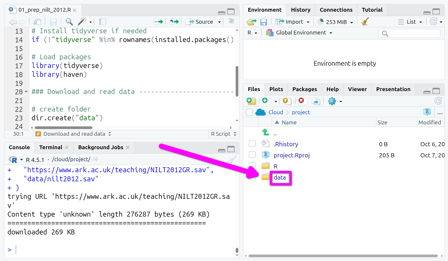
dir.create("data")

Again, with your text cursor on the dir.create(...) line of code, press Ctrl+Enter or click the run button. You should see the data folder appear in the files pane (bottom-right). (Though, if not, check whether you are still in the R sub-folder, and if so navigate back up to the parent directory.)

We now need the code to download the file with the NILT data set. We can do this by using another function we used last week, the download.file() function. The arguments for this are download.file("URL", "folder/filename.type"). So, we need a URL for where the file is available online and we need to then specify where and with what name we want to download it.

Add the following then next within your R script. As this involves a URL, it is OK to copy and paste this code rather than typing it out manually.

# Download NILT 2012
download.file(
  "https://www.ark.ac.uk/teaching/NILT2012GR.sav",
  "data/nilt2012.sav"
)

Again select the code and run it.

Take a look in the ‘Files’ tab in bottom-right, you should now have a folder called ‘data’, click on it, and you will see the nilt2012.sav file.

Remember within the Files tab to navigate back to the main project folder to also click project in the nav-bar or the .. at the top of the list of files - so, given we only have one file, right-above the nilt2012.sav.

The .sav is the SPSS file format. We will need to use a function made available to us by haven to read it into R, read_sav().

Let’s use it to read in the .sav file and assign it to an object called nilt.

# Read NILT
nilt <- read_sav("data/nilt2012.sav")

Once more, put your text cursor on the line that reads in the data and run it.

And that’s it! You should see a new data object in your ‘Environment’ tab (Pane 2 - top-right) ready to be used. If you recall last week, we read in the police_killings.csv file using read_csv(). Despite the NILT data being stored in the SPSS file-type, once read in, we can see it and interact with it the same as our data last week.

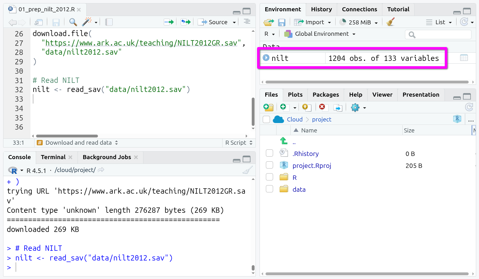
You can also see that this contains 1204 observations (rows) and 133 variables (columns). If you click on it, you can open it up in a new tab like an Excel sheet.

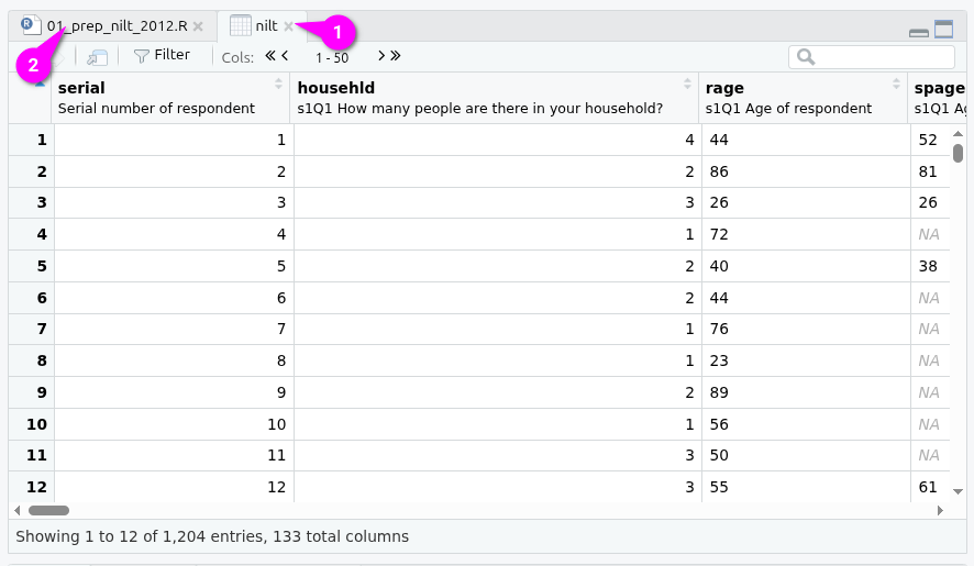
(You can get back to your R script by either (1) clicking the small ‘x’ to close the tab showing the nilt data frame or (2) clicking on the tab for the R script.)

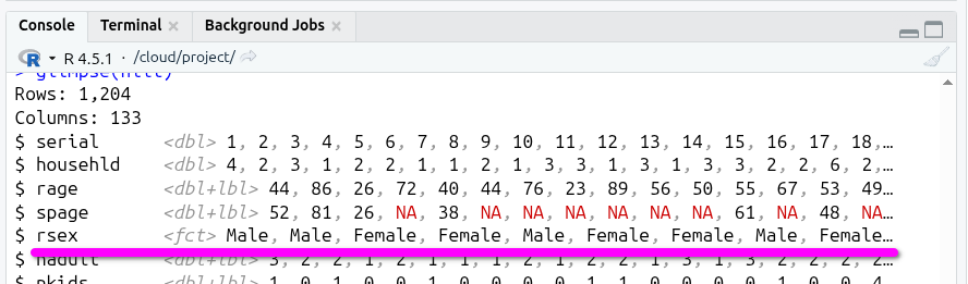
Whilst that gives us a visual interactive view of our data frame. You will notice scrolling along the columns that variables like rsex has values of 1 and 2 rather than showing the category labels. To explore this in more detail we need to switch back to code. Also, as you build up your R skills you will find it much quicker - and more intuitive - to start exploring your data using code rather than opening it up in visual views like this.

Let’s glimpse() our data frame to see the types of variables included and understand why we do not see our category labels.

As we are now moving from code we are writing so anyone with our script can setup their own R project the same as our own to taking a quick look at our data, do not add glimpse() to your R script. Instead, type the following in the Console.

glimpse(nilt)

(Being able to move from the source pane (top-left) to the Console (bottom-left) to switch between ‘writing code we want to save in our file’ and ‘writing code to quickly check our data’ is a benefit of RStudio. Whilst it may have looked intimidating at first with, all of its panes and tabs, you can hopefully now see how this supports quickly moving between different tasks.)

Data wrangling

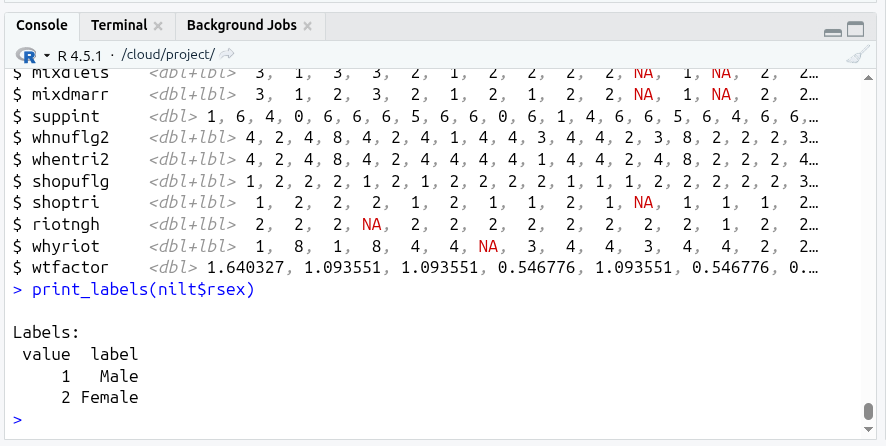
As you can see from the result of glimpse(), the class for practically all the variables is <dbl+lbl> (which if recall from last week, stands for double - i.e. numeric - and label).

What does this mean? This happened because usually datasets use numbers to represent each of the categories/levels in categorical variables. These numbers are labelled with their respective meaning. This is why we have a combination of value types (<dbl+lbl>).

Look at rsex in the glimpse() output, as you can see from the values displayed this includes numbers only, e.g. 1,1,2,2.... This is because ‘1’ represents ‘Male’ respondents and ‘2’ represents ‘Female’ respondents in the NILT dataset (n.b. the authors of this lab workbook recognise that sex and gender are different concepts, and we acknowledge this tension and that it will be problematic to imply or define gender identities as binary, as with any dataset. More recent surveys normally approach this in a more inclusive way by offering self-describe options). You can check the pre-defined parameters of the variable in NILT in the documentation or running print_labels(nilt$rsex) in your Console, which returns the numeric value (i.e. the code) and its respective label. As with rsex, this is the case for many other variables in this data set.

You should be aware that this type of ‘mix’ variable is a special case since we imported a file from a SPSS file that saves metadata for each variable (containing the names of the categories). The read_sav() function let us read this in as a data frame so we can use it in R, preserving the metadata as well. However, as with any data we load in, we still need to clean and ‘wrangle’ it to make it useable.

As you learned in the last lab, in R we treat categorical variables as factor. Therefore, we will coerce some variables as factor. This time we will use the function as_factor() instead of the simple factor() that we used before. This is because as_factor() allows us to keep the existing category labels in the variables - in other words, it will use the codes (<dbl>) and category labels (<lbl>) already in the data to turn it into a factor variable. The syntax is exactly the same as before.

Back to our R script then. First, use a comment to make clear we are starting a new section:

# Coerce variables   ---------------------------------------------------------

Next add and run the following in your script:

# Gender of the respondent
nilt <- nilt |> mutate(rsex = as_factor(rsex))
# Highest Educational qualification
nilt <- nilt |> mutate(highqual = as_factor(highqual))
# Religion
nilt <- nilt |> mutate(religcat = as_factor(religcat))
# Political identification
nilt <- nilt |> mutate(uninatid = as_factor(uninatid))
# Happiness
nilt <- nilt |> mutate(ruhappy = as_factor(ruhappy))

Notice from the code above that we assign the result of mutate() back to our nilt data frame, the nilt <- ... part of the code. This replaces our ‘old’ data frame with a version with the mutated variables that are of type factor.

Back in the Console again, run glimpse(nilt) once more and scroll up to see the line for rsex in the output.

R has taken the codes (the <dbl> values) and mapped them to the labels (the <lbl> values), whereby we can now more easily see and work with our categories.

Last week, with the police killings data we could simply use factor() on our variables as the values were saved in the file as category labels without any codes. The data for it was stored in a CSV file, that does not store metadata mapping codes and category labels. As a way around that limitation, some data made available via CSV files will store categorical variable values as labels only, with no codes. Running factor() in such cases creates codes for each unique label. The only danger with that, and something to keep eye out for, is any typos in the data, such as Scotland and Scoltand, as they are ‘unique’ labels would result in these being treated as two different categories after running factor().

If we read in our data from a file type that stored the values as codes, but did not include the metadata for category labels, we would instead need to manually add this mapping, along the lines of:

survey <- survey |>
  mutate(
    country = factor(
      country,
      levels = c(1, 2),
      labels = c("Scotland", "England")
    )
  )

Back to our NILT data again - What about the numeric variables? In the NILT documentation (covered in later section) there is a table in which you will see a type of measure ‘scale’. This usually refers to continuous numeric variables (e.g. age or income).² Let’s coerce some variables to the appropriate numeric type.

In the previous operation we coerced the variables as factor one by one, but as covered at the end of last week’s lab we can also transform several variables at once within a single mutate function.

Add and run the following code in your script:

# Coerce several variables as numeric
nilt <- nilt |>
  mutate(
    rage = as.numeric(rage),
    rhourswk = as.numeric(rhourswk),
    persinc2 = as.numeric(persinc2),
  )

Another thing we need to do is drop any unused levels (or categories) in our dataset using the function droplevels(), by adding and running the following in our script:

# drop unused levels
nilt <- droplevels(nilt)

This function is useful to remove some categories that are not being used in the dataset (e.g. categories that have 0 observations).

Finally, as we now have our data and done some wrangling, we do not want to have to repeat it each time we load the data in our R Markdown files. So, let’s save it as an .rds file - R’s own file-type.

This will save us time in future labs, as we will be able to read in an already formatted version of the NILT in future labs.

Add a comment then to make clear we have a new section:

# Save data ------------------------------------------------------------------

Then add and run the code to save our nilt data frame as an RDS file.

# save as rds
saveRDS(nilt, "data/nilt_r_object.rds")

Lastly, as this script is merely to download, prep, and save a cleaned version of our data, it is good practice to end by clearing the global environment. This removes all loaded objects and puts it can into a clear state. We do this for a few reasons, including (1) if we did more complex setup operations the global environment could be filled with a lot of objects we no longer need, and (2) whilst we will continue naming the object containing our data frame as ‘nilt’ in the labs, we would not want to enforce this on anyone we share the project with.

Add and run then the following at the end of your R script:

# clean global environment
rm(list=ls())

You should now see your Global Environment is empty:

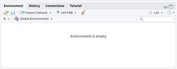
Note, whilst this removes objects, like our nilt data frame, it does not remove any loaded libraries, so the functions provided by the tidyverse and haven remain available to us after running this line of code.

The NILT Documentation

Please take 5-10 minutes to read the documentation for the dataset. Such documentation is always important to read as it will usually cover the research design, sampling, and information on the variables. For instance, page 7 onwards has the codebook with columns listing variable name, variable label, values, and measure. Page 6 of the documentation provides a “Navigating the codebook (example section)” overview for how to understand the table.

It is also worthwhile taking a look through the questionnaires for the survey as well. You will have to regularly consult the technical document and questionnaires to understand and use the data in the NILT data set. So, I recommend you to bookmark the links / save copies of the PDF files.

This NILT teaching dataset is also what you will be using for the research report assignment in this course (smart, isn’t it?) - so it’s worth investing the time to learn how to work with this data through the next few labs, as part of the preparation and practice for your assignment.

(Aside: Best practice would be to read through key info in the documentation first before downloading and coercing variables - we have done the inverse today solely to ensure you have adequate time within the lab itself to download and prepare the data.)

Variable Names and Labels

Let’s first go through the codebook in more detail. This will help you understand how to read the information in it, and some common ‘gotchas’ to look out for.

The “Variable Name” is how the variables are named in the data set - except in all caps, whereas once we start working with the data they will be lowercase. If we read the data set into a data frame named nilt, the rage variable name would be accessed as nilt$rage. For consistency with how they will appear when working with them in R, we will stick to using all lower case in the lab workbook.

The “Label” column mostly shows the corresponding text used in the survey for the variable. For rage it is “Q1. Household grid: Age of respondent”. If you look at page 2 of the main questionnaire, you will see that the ‘household grid’ was a repeat set of questions used to gather key information about each member of the household. The r in rage stands for “respondent”, i.e. the person who answered the survey questions.

Some variable names, such as work and tunionsa on page 9, note under the name “(compute)”. This means the variable rather than representing a direct answer to a survey question is instead ‘computed’ / ‘derived’ from answers to other questions. The variable label for these then detail which questions were used to compute these variables. Work status may seem an odd variable to compute rather than ask directly.

However, if we look at work, we can see from page 39 in the main questionnaire, a series of questions were asked to ascertain employment status and economic activity. Given the diversity of situations people can be in, it is more practical to ask a series of yes/no and other questions and then use these to calculate categories for other variables.

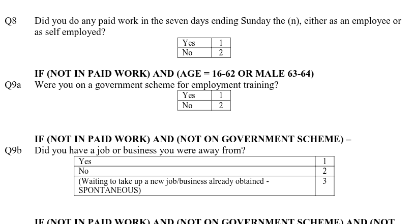
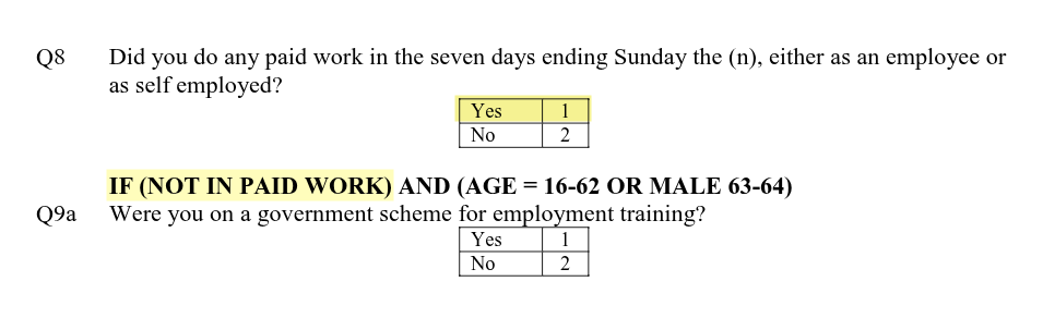
Whilst it may look more complex having all these questions on paper, it is simpler for respondents. Let’s imagine being a 32 year old respondent who answers ‘No’ to Q8, whether taken part in paid work in last seven days, and then ‘Yes’ to Q9a, whether taking part in a government scheme for employment training.

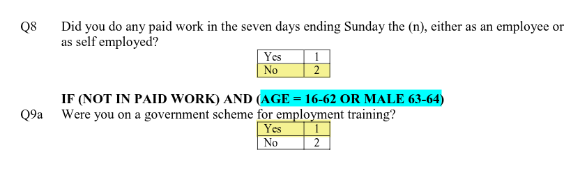
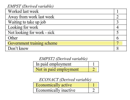
From these two answers we can compute the respondent is ‘Government training scheme’ for empst, ‘Not in paid employment’ for empst2, and ‘Economically active’ for econact. Note as well that Q9a was only asked based on whether the participant would be eligible for the government training scheme, calculated using age and gender. (Highlighted in blue above.)

Importantly, we gathered this information by asking simple yes/no questions, structured the questions in way to only ask the minimum number of questions relevant for the respondent, and avoided needing to explain jargon such as ‘economically active’. Economically active means someone is either in employment (including waiting to start a job they have been offered and accepted) or unemployed but looking for work and if offered could start a job within the next two weeks. Imagine now asking a respondent whether they are economically active and then having to explain what that means and figuring out whether they are or not. The way the survey questions are structured captures this complexity - and more - and all without ever having to provide a definition of economically active.

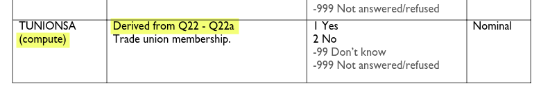
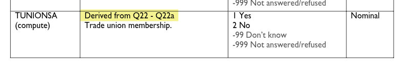
The tunionsa variable is also a good example of we why cannot assume what a variable measures by its name alone. As can see bottom of page 9 in the documentation, tunionsa is derived from Q22 and Q22a.

However, if we look at those two questions on page 43 of the questionniare - screenshot below to save having to switch tabs - we can see Q22 asks the respondent whether they are currently a member of a trade union or staff association and Q22a is whether they have ever been a member.

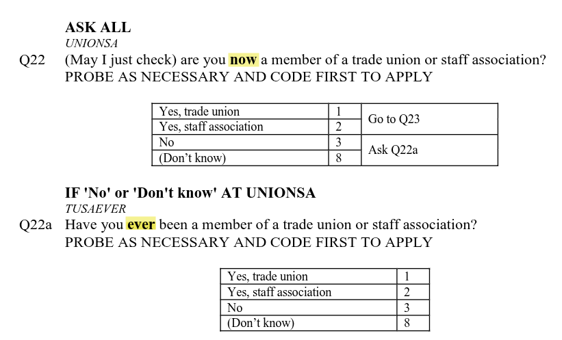
If a respondent answered ‘Yes, trade union’ or ‘Yes, staff association’ for either Q22 or Q22a the value computed for tunionsa is ‘Yes’. Whilst tunionsa then is broadly a measure of trade union membership it would be more accurate to say it is a measure of whether the respondent currently is or ever was a member of a trade union or staff association.

Do not worry if you could not tell that from just the codebook. Normally, dataset documentation should also include a separate section with information on how each computed variable was derived. I was only able to confirm this was how tunionsa was computed by checking the values with those for Q22 and Q22a in the main data set. Expectations of what documentation for data sets should include are continuing to improve over time. However, whilst you should encounter such situations less often with newer data sets, it can still remain unclear - where you may need to do your own additional checks, or contact the original researchers to clarify.

This though does show the importance of not assuming what a variable measures by just its name and label. If we mistook tunionsa as measuring current membership only, we may then later be surprised seeing the high number of people currently unemployed with ‘Yes’ for tunionsa. It is not surprising to see that though when we understand that ‘Yes’ includes those who have ever been a member.

Values and Measures

The ‘Measure’ column in the codebook tells us whether the variable is ‘scale’, ‘nominal’, or ‘ordinal’. This is based on how SPSS, the proprietary statistical analysis program that was used by the NILT project, stores variables. Within R, these correspond respectively with numeric, (unordered) factor, and ordered factor variables that we covered last week. As we covered earlier in the lab, the tidyverse also provides us with tools to work with data created in SPSS.

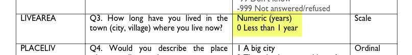
The ‘Values’ column then tells us what the numbers represent. For numeric variables this is the unit being measured, such as “years” and “number of people”. This may seem ‘obvious’ for some variables, but good documentation should still always provide this information. The importance of this becomes clearer if we look at livearea. Without it clarifying “Numeric (years)” someone could mistake it as representing number of months instead. Similarly, the “0 Less than 1 year” is an important clarifier, helping us understand that anything less than 1 year was recorded as 0. In other words, if someone had lived in the area for 7 months, it was still recorded as 0 rather than rounded up to 1.

For the categorical variables it then provides the code and label for the categories. For example, with rsex the categories are 1 (code) Male (label) and 2 (code) Female (label). As mentioned last week, the ‘raw’ data is often stored in numeric codes as - among other reasons - it is more efficient to store it this way. Using the codebook, someone looking at the raw data would then know that a value of 1 represents Male. And as we covered above, knowing the code and label means we can set up the data in R to show the labels instead of the raw codes. (And if we were working with data in a file with only the codes and not the labels, we can use the codebook to write our own code to map codes and labels.)

You may have spotted though that the Values column for some variables also includes additional grey text, “-9 Non Applicable”, “-99 Don’t Know”, and “-999 Not answered/refused”. These are part of what is known as ‘missing values’, where we do not have an answer to a question for a participant, where these values record the reason why an answer is missing. Recording such reasons is important for multiple reasons. Let’s take ‘-9 Non Applicable’, which following convention is used in the NILT to denote the reason there is no answer is the participant was not asked the question. For example, as shown in image below if a person answered ‘Yes’ to question 8 to say they were in paid work, then they were not asked question 9a.

For clarity, we record it as ‘non applicable’ instead of leaving it blank or ‘No’. If we left it blank we would not know whether it was blank because the question was skipped deliberately or accidentally. If we recorded it as ‘No’ rather than ‘non applicable’, we lose distinction between our participants. For instance, say we had 100 respondents and 10 answered yes, 20 answered no, and 70 were non applicable. We know from those values that of the 30 who could potentially be on a government scheme 20 were not.

“-99 Don’t Know” and “-999 Not answered/refused” are then useful to know whilst the question was applicable to the respondent, it was not answered for another reason. During a pilot of the survey, a higher than expected number of “Don’t know” and “Not answered” can also help indicate where a question is potentially unclear or phrased in a way that respondents do not feel comfortable answering.

Importantly though as ‘missing values’ they are treated the same in analysis. Within R, values designated as ‘missing values’ are grouped together and labelled “NA”. Take note, this stands for “Not available” - covering all reasons a value is not available (i.e. missing). A common mistake people make is to assume NA stands for ‘non applicable’, resulting in inaccurate interpretations.

As with all conventions though, there are situations where it can be useful to not treat certain values as ‘missing’. Whilst the NILT treats “Don’t know” as a missing value, some surveys will have questions where “Don’t know” is a meaningful answer for the analysis. For example, with a question like “Who is the current UK Prime Minister?” as part of research on public understanding of politics, a “Don’t know” is a meaningful answer rather than a missing value. In such cases, the “Don’t know” would not have a “-99” or equivalent code.

In some cases it can also be worthwhile exploring whether there is any pattern behind missing values. It may turn out that certain groups were more likely to refuse to answer or respond “Don’t know” to specific questions. This can then open discussion as to why and what changes to the survey design may help address it. Again that we record the reason the value is ‘missing’ rather than leaving the value blank makes it possible to still do that.

Read the clean dataset

Phew! Good job. You have completed the basics for wrangling the data and producing a workable dataset and gone through the documentation to understand it better.

As a final step, just double check that things went as expected. For this purpose, we will re-read the clean dataset in the Activities below.

First though, let’s set up a new R Markdown file you can use for the Activities. Within the ‘Files’ pane (bottom-right):

1. Click ‘New file’
2. Click ‘R Markdown’

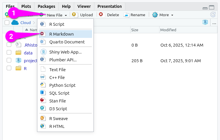
This will open a dialogue for creating a new file:

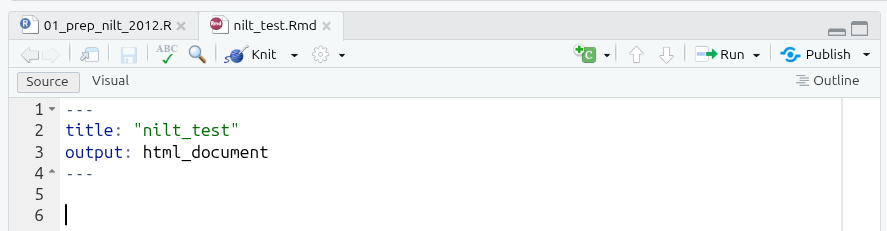
4. Add nilt_test.Rmd as the new file name.
5. Click the OK button to confirm creation of an R Markdown file.

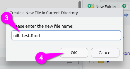
This will create the file and open it in a new tab:

You are now ready for the activities for the end of this week’s lab.

Activities

• Within your R Markdown file create a code chunk to load the tidyverse and haven packages.

(Aside: Whilst we saved our file as .rds as the original file was .sav we still need to load haven to read all the information stored in it. These packages also remain in our environment, but this ensures our R Markdown file will still run without issue if we restart our R session.)

• Using the readRDS() function, create a code chunk and:

  1. read the .rds file that you just created in the last step and assign it to an object called cleaned_nilt. (Hint: You need to read it in by providing “folder/file-name.rds” as an argument.)
  2. read in the original .sav file that we downloaded and assign it to an object called unclean_nilt.

• Run the glimpse function on the cleaned_nilt object.

• Run the glimpse function on the unclean_nilt object.

• Do they look the same? (If yes, it means that you successfully saved a version of the nilt data with our coerced variables.)

• Finally, write code in the Console to clean your global environment, so we have a clear environment to start with next week.

---

An Aside About File-Types

(This is a lengthy aside providing more info on file-types for those interested, it is optional to read.)

File-types like CSV and TSV are what is known as ‘interoperable’, meaning they are not limited to a specific app. Ideally then this is the file-type data should be shared in to support openness, transparency, and reproducibility.

However, as covered in the online lecture this week, CSV does not store ‘metadata’. If using 1, 2, 3, … codes for a categorical variable, this information is stored separately, and if loading in data requires mapping codes and labels (e.g. 1 = UK, 2 = France, …). This can quickly become tedious and time-consuming. Whilst various attempts have been made to create ‘data packaging formats’ that build on top of CSV and/or TSV, none have gained wide-spread popularity. As a result, it is still common to see data being shared in data archives as an SPSS and/or Stata file - sometimes with a CSV file as well. (Some archives also auto-convert data into SPSS and Stata file type versions to download.)

Decades ago, data being in the SPSS file type would have forced you to use - and pay an expensive license for - SPSS. To help end this situation many researchers found themselves within, The Free Software Foundation (FSF) created ‘PSPP’, a free alternative to SPSS, that can read and save to the same SPSS sav file-type. And, it is code from ‘PSPP’ that haven uses to read SPSS files. This involved pain-staking work ‘reverse engineering’ the SPSS file-type to understand how the data is stored and writing code so that other software - and not just SPSS - could use it. It was then not SPSS’s benevolence that made it possible to read SPSS files in R - indeed, proprietary software companies often do all they can to prevent other software being able to use their proprietary file-types. It was instead the work of an open community striving to ensure people have freedom in how they use their computers and are not forced into using specific software. (Sadly, for all the good they do, the FSF likes giving their projects terrible names, with PSPP not actually standing for anything, it is instead the ‘inverse’ of SPSS, playing on it being a free open alternative to proprietary closed software.)

Indeed, PSPP and haven are the victims of their own success here. With the haven package, it does not matter that the data is in a proprietary SAS, SPSS, or Stata file type, it can be read into R. Importantly, it can be read into R in a way that can then immediately start being used with all the core tidyverse functions.

Despite SPSS files being a closed proprietary format then, because it is easy to read the data into R and it maintains metadata, a lot of researchers and data archives use it as if it were an open file type, using it still to archive data. This has likely contributed to the lack of widespread adoption of the open data packages aiming to replace the proprietary file formats, as having an alternative way to share data is not a pressing need. However, I would still encourage you if looking to archive your own data in future to consider ways in which you can make it available using a proper open standard.

Footnotes

1. Another way to do this is using the renv package. This package creates a unique separate environment, including for installed packages, for each project you are working on. If you were using RStudio Desktop and were working on analysis projects that required different specific versions of the same packages, renv makes that possible as it creates a folder with the installed packages for each project. Even when working on a single project as renv maintains a record of which version of a package was used this is more ‘future-proof’. If a package used made major changes, renaming functions or changing how arguments are passed to them, the code may no longer work. renv though would retrieve and install the exact same version as originally used, helping ensure it will run now and well into the future.

2. Be careful, in some cases these actually correspond to discrete numeric values in this dataset (things that can be counted, e.g. number of…).