Workbook suggested answers

Introduction

This chapter presents the suggested R code to answer the workbook activities and exercises throughout the course labs in Quantitative Methods in the Social Sciences. This covers Lab 3 to Lab 10.

Before looking at the answers, try asking your tutor for help. Also, we strongly recommend web resources, such as https://stackoverflow.com/ or https://forum.posit.co/. By solving the issues, you will learn a lot! ;)

Lab 3. Data wrangling

## Load the packages
library(tidyverse)
library(haven)

# Read the cleaned data from the .rds file
cleaned_nilt <- readRDS("data/nilt_r_object.rds")
# Read the original .sav file
unclean_nilt <- read_sav("data/nilt2012.sav")

# Glimpse both
glimpse(cleaned_nilt)
glimpse(unclean_nilt)

The two data frames should not look the same. In cleaned_nilt the eight variables we coerced (rsex, highqual, religcat, uninatid and ruhappy as <fct>; rage, rhourswk and persinc2 as <dbl>) show their category labels or plain numbers, whereas in unclean_nilt every variable is still <dbl+lbl>. If they look identical, the coerced version was not saved.

Lab 4. Exploratory data analysis

Preamble code

## Load the packages
library(tidyverse)
# Read the data from the .rds file
nilt <- readRDS("data/nilt_r_object.rds")

# Subset
nilt_subset <- nilt |> 
  select(rsex, rage, highqual, religcat, uninatid, ruhappy, rhourswk, persinc2)

Activity 1

In your R Markdown file, do the following activities using the data stored in the nilt_subset object:

• Create a One-Way contingency table for uninatid in the nilt_subset dataset using the sumtable() function;

# Load the vtable package to create summary tables
library(vtable)
# Create table
sumtable(nilt_subset, vars = c("uninatid"))

Summary Statistics

Variable	N	Percent
uninatid	1183
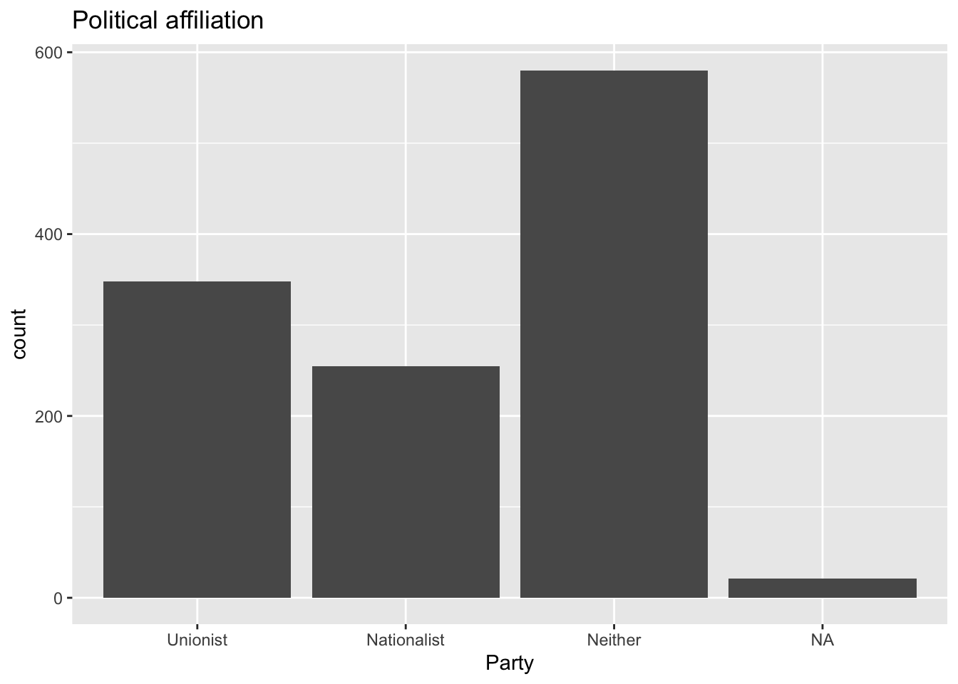
... Unionist	348	29%
... Nationalist	255	22%
... Neither	580	49%

• Using the variables religcat and uninatid, generate a Two-Way contingency table;

sumtable(nilt_subset, vars = c("religcat"), group = "uninatid")

Summary Statistics

uninatid	Unionist		Nationalist		Neither
Variable	N	Percent	N	Percent	N	Percent
religcat	341		255		558
... Catholic	2	1%	245	96%	238	43%
... Protestant	305	89%	5	2%	180	32%
... No religion	34	10%	5	2%	140	25%

Activity 2

Using the data in the nilt_subset object, complete the following activities.

• Using the hist() function plot a histogram of personal income persinc2. From the NILT documentation this variable refers to annual personal income in £ before taxes and other deductions;

hist(nilt_subset$persinc2)

• Create a summary of the personal income persinc2 variable, using the sumtable() function.

sumtable(nilt_subset, vars = c("persinc2"))

Summary Statistics

Variable	N	Mean	Std. Dev.	Min	Pctl. 25	Pctl. 75	Max
persinc2	897	16395	13466	260	6760	22100	75000

• Compute the mean and standard deviation of the personal income persinc2, grouped by happiness ruhappy.

sumtable(nilt_subset, vars = c("persinc2"), group = "ruhappy")

Summary Statistics

ruhappy	Very happy			Fairly happy			Not very happy			Not at all happy			Can't choose
Variable	N	Mean	SD	N	Mean	SD	N	Mean	SD	N	Mean	SD	N	Mean	SD
persinc2	305	17569	13429	500	16262	14015	62	13445	9754	9	12451	11501	15	11457	6113

Lab 6. Visual exploratory analysis

Preamble code

## Load the packages
library(tidyverse)

# Load the data from the .rds file we created in the last lab
nilt <- readRDS("data/nilt_r_object.rds")
# Create subset
nilt_subset <- nilt |>
  select(rsex, rage, highqual, religcat, uninatid, ruhappy, rhourswk, persinc2)

Activity

Using the nilt_subset object, complete the tasks below in the ‘Lab-6-Visual.Rmd’ file, which you created earlier. Insert a new chunk for each of these activities and include brief comments as text in the Rmd document to introduce the plots and discuss the results (tip —leave an empty line between your text and the next chunk to separate the description and the plots):

• Create a first-level header to start a section called “Categorical analysis”;

# Categorical analysis

• Create a simple bar plot using the geom_bar() geometry to visualize the political affiliation reported by the respondents using the variable uninatid;

ggplot(nilt_subset, aes(x = uninatid)) +
  geom_bar() +
  labs(title = "Political affiliation", x = "Party")

• Based on the plot above, create a ‘stacked bar plot’ to visualize the political affiliation by religion, using the uninatid and religcat variables;

ggplot(nilt_subset, aes(x = uninatid, fill = religcat)) +
  geom_bar() +
  labs(
    title = "Political affiliation by religion",
    x = "Party", fill = "Religion"
  )

• Create a new first-level header to start a section called “Numeric analysis”;

# Numeric analysis

• Create a scatter plot about the relationship between personal income persinc2 on the Y axis and number of hours worked a week rhourswk on the X axis;

ggplot(nilt_subset, aes(x = rhourswk, y = persinc2)) +
  geom_point() +
  labs(
    title = "Income and number of hours worked a week",
    x = "Number of hours worked a week", y = "Personal income (£ a year)"
  )

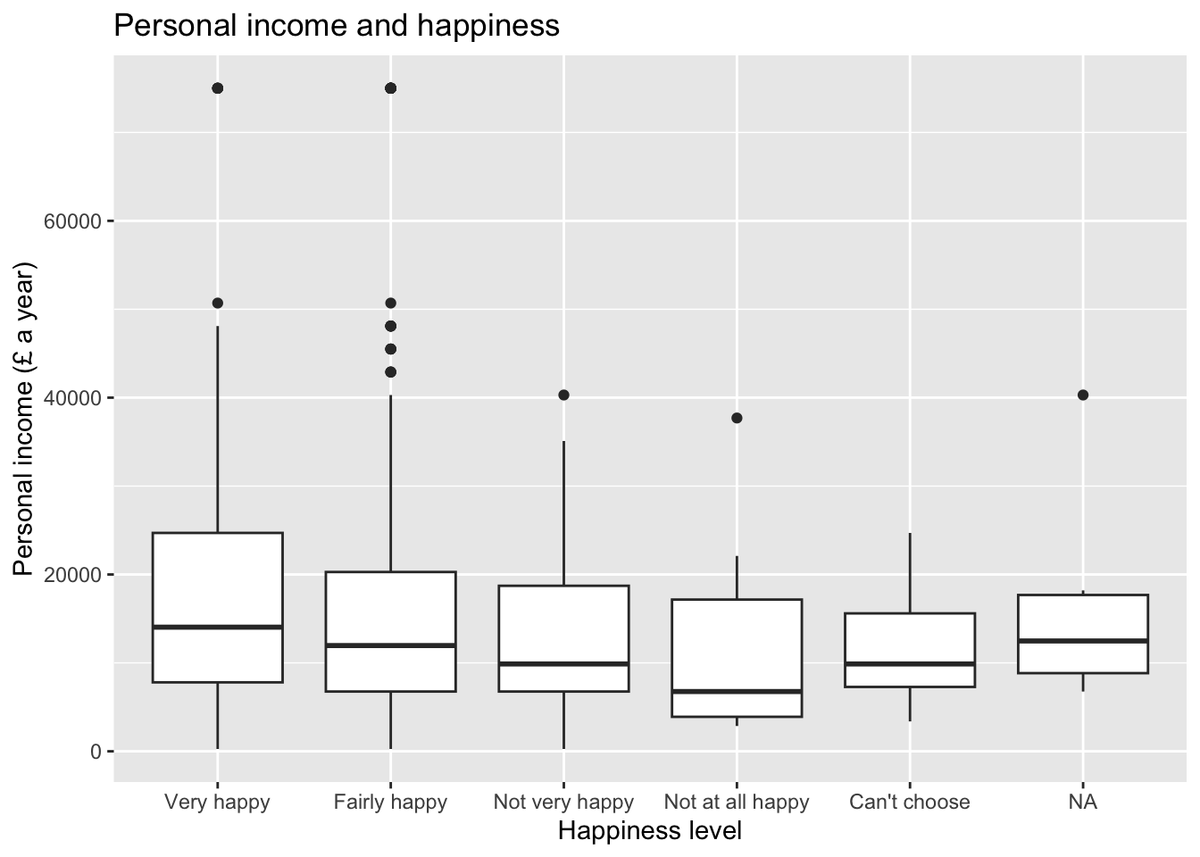
• Finally, create a box plot to visualize personal income persinc2 on the Y axis and self-reported level of happiness ruhappy on the x axis… Interesting result, Isn’t it? Talk to your neighbour or tutor about your results;

ggplot(nilt_subset, aes(x = ruhappy, y = persinc2)) +
  geom_boxplot() +
  labs(
    title = "Personal income and happiness",
    x = "Happiness level", y = "Personal income (£ a year)"
  )

• Briefly comment each of the plots as text in your Rmd file;
• Knit the .Rmd document as HTML. The knitted file will be saved automatically in your project. You can come back to the Rmd file to make changes if needed and knit it again as many times as you wish.

Lab 7. Correlation

## Load the packages
library(tidyverse)
library(haven)
# Load the data from the .rds file we created in lab 3
nilt <- readRDS("data/nilt_r_object.rds")

# Age of respondent’s spouse/partner
nilt$spage <- as.numeric(nilt$spage)
# Migration
nilt <- mutate_at(nilt, vars(mil10yrs, miecono, micultur), as.numeric)

# overall perception towards migrants
nilt <- rowwise(nilt) |>
  # sum values
  mutate(mig_per = sum(mil10yrs, miecono, micultur, na.rm = T)) |>
  ungroup() |>
  # assign NA to values that sum 0
  mutate(mig_per = na_if(mig_per, 0))

Activity 1

Using the nilt data object, visualize the relationship of the following variables by creating a new chunk. Run the chunk individually and comment on what you observe from the result as text in the Rmd file (remember to leave an empty line between your text and the chunk).

• Create a scatter plot to visualize the correlation between the respondent’s overall opinion in relation to migration mig_per and the respondent’s age rage. Remember that we just created the mig_per variable by summing three variables which were in a 0-10 scale (the higher the value, the better the person’s perception is). In aes(), specify rage on the X axis and mig_per on the Y axis. Use the ggplot() function and geom_point(). Also, include a straight line describing the points using the geom_smooth() function. Within this function, set the method argument to 'lm'.

nilt |> ggplot(aes(x = rage, y = mig_per)) +
  geom_point() +
  geom_smooth(method = "lm") +
  labs(
    title = "Perception of migration vs age",
    x = "Respondent age", y = "Perception of migration (0-30)"
  )

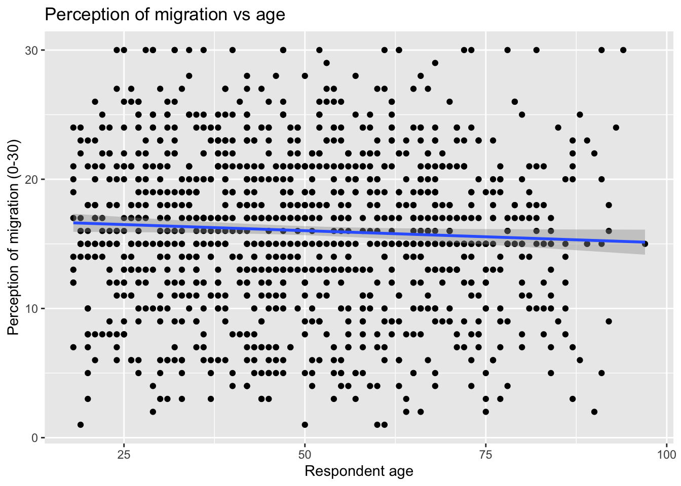
• What type of relationship do you observe? Comment the overall result of the plot and whether this is in line with your previous expectation.

Activity 2

• Create a boxplot to visualize the relationship between the respondent’s overall opinion in relation to migration mig_per (Y axis) and constitutional view uninatid (X axis).

nilt |> ggplot(aes(x = uninatid, y = mig_per)) +
  geom_boxplot() +
  labs(
    title = "Perception of migration by constitutional view",
    x = "Constitutional view", y = "Perception of migration (0-30)"
  )

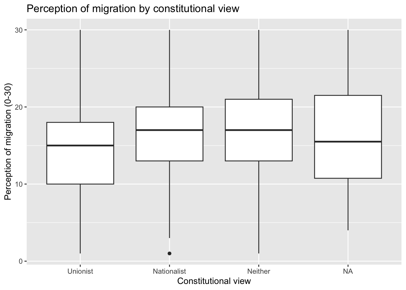
• Do you think the opinion towards migration differs among the groups? Re: The boxes overlap considerably, but unionist respondents have a slightly lower median (15) than nationalist respondents and those identifying with neither (17 for both). So there is a modest difference in the overall perception of migration between the groups, with a lot of variation within each group.

Activity 3

• Compute a correlation matrix for rage, persinc2, mil10yrs, miecono and micultur, using 'pairwise.complete.obs' and rounding to 3 decimals.

nilt |>
  select(rage, persinc2, mil10yrs, miecono, micultur) |>
  cor(use = "pairwise.complete.obs") |>
  round(3)

           rage persinc2 mil10yrs miecono micultur
rage      1.000   -0.036   -0.024  -0.029   -0.099
persinc2 -0.036    1.000    0.165   0.199    0.195
mil10yrs -0.024    0.165    1.000   0.716    0.627
miecono  -0.029    0.199    0.716   1.000    0.665
micultur -0.099    0.195    0.627   0.665    1.000

• Is personal income or age correlated with the perception of migrants? Re: Age is not correlated with any of the three migration variables (all coefficients are close to 0, between -0.02 and -0.10). Personal income shows a weak positive correlation with all three (around 0.17 to 0.20): respondents with higher incomes tend to report slightly more positive views of the effects of migration on the economy (miecono), on culture (micultur) and on Northern Ireland over the last ten years (mil10yrs). The three migration variables are strongly correlated with each other (0.63 to 0.72), which is why combining them into mig_per is reasonable.

Lab 8. Linear model. Simple linear regression

## Load the packages
library(tidyverse)
# Read the data from the .rds file
nilt <- readRDS("data/nilt_r_object.rds")

m3 <- lm(persinc2 ~ rhourswk, data = nilt)

Lab activities

Use the nilt data set object in your ‘Lab-8-Simple-Linear-Regression.Rmd’ file to:

1. Plot a scatter plot using ggplot. In the aesthetics, locate rhourswk in the X axis, and persinc2 in the Y axis. In the geom_point(), jitter the points by specifying the position = 'jitter'. Also, include the best fit line using the geom_smooth() function, and specify the method = 'lm' inside.

ggplot(nilt, aes(x = rhourswk, y = persinc2)) +
  geom_point(position = "jitter") +
  geom_smooth(method = "lm")

2. Print the summary of m3 using the summary() function.

summary(m3)

Call:
lm(formula = persinc2 ~ rhourswk, data = nilt)

Residuals:
   Min     1Q Median     3Q    Max 
-43694  -8148  -3070   4990  58249 

Coefficients:
            Estimate Std. Error t value Pr(>|t|)    
(Intercept)   5170.4     1966.2    2.63  0.00884 ** 
rhourswk       463.2       52.4    8.84  < 2e-16 ***
---
Signif. codes:  0 '***' 0.001 '**' 0.01 '*' 0.05 '.' 0.1 ' ' 1

Residual standard error: 13860 on 455 degrees of freedom
  (747 observations deleted due to missingness)
Multiple R-squared:  0.1466,    Adjusted R-squared:  0.1447 
F-statistic: 78.15 on 1 and 455 DF,  p-value: < 2.2e-16

3. Is the relationship of hours worked a week significant? Re: Yes. The p-value (fourth column of the ‘Coefficients’ table) is lower than 0.05.
4. What is the adjusted r-squared? How would you interpret it? Re: the adjusted R-squared is 0.14. This can be interpreted in terms of percentage, e.g. 14% of the variance in personal income can be explained by the number of hours worked a week.
5. What is the sample size to fit the model? Re: The total number of observations in the data set is 1,204 and the model summary says that 747 observations were deleted due to missingness. Therefore, the sample size is 457 (1204-747).
6. What is the expected income in pounds a year for a respondent who works 30 hours a week according to coefficients of this model?

5170.4 + 463.2 * 30

[1] 19066.4

7. Plot a histogram of the residuals of m3 using the residuals() function inside hist(). Do the residuals look normally distributed (as in a bell-shaped curve)?

hist(residuals(m3))

Overall, the residuals look normally distributed with the exception of the values to the right-hand side of the plot (between 40000 and 60000).

Lab 9. Multiple linear regression (part 1)

Lab activities

Load the packages and the data that you will need in your file using the code below:

## Load the packages
library(moderndive)
library(tidyverse)
# Read the data from the .rds file
nilt <- readRDS("data/nilt_r_object.rds")

1. Print a table for the highest level of qualification highqual using the table() function.

table(nilt$highqual)

Degree level or higher       Higher education   GCE A level or equiv 
                   230                    102                    243 
     GCSE A-C or equiv      GCSE D-G or equiv      No qualifications 
                   185                     82                    281 
  Other, level unknown           Unclassified 
                    27                     54 

2. Generate a scatter plot using ggplot. Within aes(), locate the number of hours worked a week rhourswk on the X axis and the personal income persinc2 on the Y axis, and specify the color of the dots by the highest level of qualification highqual. Use the geom_point() function and ‘jitter’ the points using the argument position. Add the parallel slopes using the geom_parallel_slopes() function and set the standard error se to FALSE. What is your interpretation of the plot? Write down your comments to introduce the plot.

ggplot(nilt, aes(x = rhourswk, y = persinc2, color = highqual)) +
  geom_point(position = "jitter") +
  moderndive::geom_parallel_slopes(se = FALSE) +
  labs(
    title = "Personal income",
    subtitle = "Personal income and number of hours worked a week by education level",
    x = "Number of hours worked a week", y = "Personal income (£ a year)",
    color = "Highest education level"
  )

3. Fit a linear model using the lm() function to analyse the personal income persinc2 using the number of hours worked a week rhourswk, the highest level of qualification highqual, and the age of the respondent rage as independent variables. Store the model in an object called m4 and print the summary.

m4 <- lm(persinc2 ~ rhourswk + rage + highqual, nilt)
summary(m4)

Call:
lm(formula = persinc2 ~ rhourswk + rage + highqual, data = nilt)

Residuals:
   Min     1Q Median     3Q    Max 
-36228  -6425  -1411   4635  54749 

Coefficients:
                              Estimate Std. Error t value Pr(>|t|)    
(Intercept)                    3904.64    2714.25   1.439    0.151    
rhourswk                        444.79      45.32   9.814  < 2e-16 ***
rage                            236.59      48.47   4.881 1.47e-06 ***
highqualHigher education      -8164.91    1939.50  -4.210 3.09e-05 ***
highqualGCE A level or equiv -12439.26    1563.42  -7.956 1.47e-14 ***
highqualGCSE A-C or equiv    -13037.47    1703.07  -7.655 1.20e-13 ***
highqualGCSE D-G or equiv    -11622.07    2665.38  -4.360 1.61e-05 ***
highqualNo qualifications    -12968.10    2339.78  -5.542 5.11e-08 ***
highqualOther, level unknown  15445.70    3334.75   4.632 4.76e-06 ***
highqualUnclassified         -12399.58    2786.16  -4.450 1.08e-05 ***
---
Signif. codes:  0 '***' 0.001 '**' 0.01 '*' 0.05 '.' 0.1 ' ' 1

Residual standard error: 11830 on 447 degrees of freedom
  (747 observations deleted due to missingness)
Multiple R-squared:  0.3887,    Adjusted R-squared:  0.3764 
F-statistic: 31.58 on 9 and 447 DF,  p-value: < 2.2e-16

4. Comment on the results of the model by mentioning which of the variables is significant and their respective p-value, the adjusted r-squared of the model, and the number of observations used to fit the model. Re: All the independent variables including the number of hours worked a week, age, and all the categories of highest qualification level compared to ‘Degree level or higher’ are significant to predict personal income in the model ‘m4’, considering that the p-value is lower than 0.05. We can confirm this from the fourth column of the ‘Coefficients’ table. The adjusted R-squared of the model is 0.38 (0.3764 in the output). This means that 37.6% of the variance in personal income can be explained by these variables. The size of the sample used to fit this model is 457, considering that the ‘nilt’ data set contains 1204 observations but 747 were deleted due to missingness (1204 - 747).

Lab 10. Multiple linear regression (part 2)

Returning to the model m4 from the Lab 9 activities:

1. Comment on the R2, adjusted R2, and F-statistic to interpret the model fit. Re: The R2 is 0.389 and the adjusted R2 is 0.376, so the number of hours worked, age and highest qualification together explain around 38% of the variation in personal income among the respondents in the model. The F-statistic is 31.6 on 9 and 447 degrees of freedom with a p-value far below 0.05, so the model as a whole is statistically significant - the independent variables explain more variation than would be expected by chance.
2. How many observations were removed due to missing values? Which variables are contributing to this? Re: 747 observations were deleted due to missingness, leaving 457 of the 1,204 respondents. We can check where the missing values come from by counting the NAs in each variable:

nilt |>
  select(persinc2, rhourswk, rage, highqual) |>
  summary()

    persinc2        rhourswk           rage                         highqual  
 Min.   :  260   Min.   :  4.00   Min.   :18.00   No qualifications     :281  
 1st Qu.: 6760   1st Qu.: 25.25   1st Qu.:35.00   GCE A level or equiv  :243  
 Median :11960   Median : 37.00   Median :48.00   Degree level or higher:230  
 Mean   :16395   Mean   : 35.09   Mean   :49.62   GCSE A-C or equiv     :185  
 3rd Qu.:22100   3rd Qu.: 40.00   3rd Qu.:64.00   Higher education      :102  
 Max.   :75000   Max.   :100.00   Max.   :97.00   GCSE D-G or equiv     : 82  
 NAs    :307     NAs    :638      NAs    :3       (Other)               : 81  

Most of the missing values come from rhourswk (638 NAs, as the question was only asked of respondents in work) and persinc2 (307 NAs), with only 3 missing ages and no missing qualifications. As discussed in Lab 10, this means the model only describes respondents who are in work and reported their income, which needs to be borne in mind when interpreting the results.

3. Plot a histogram of the residuals for model m4. Do they look normally distributed? Can we trust our estimates or would you advise to carry out further actions to verify the adequate interpretation of this model?

hist(residuals(m4))

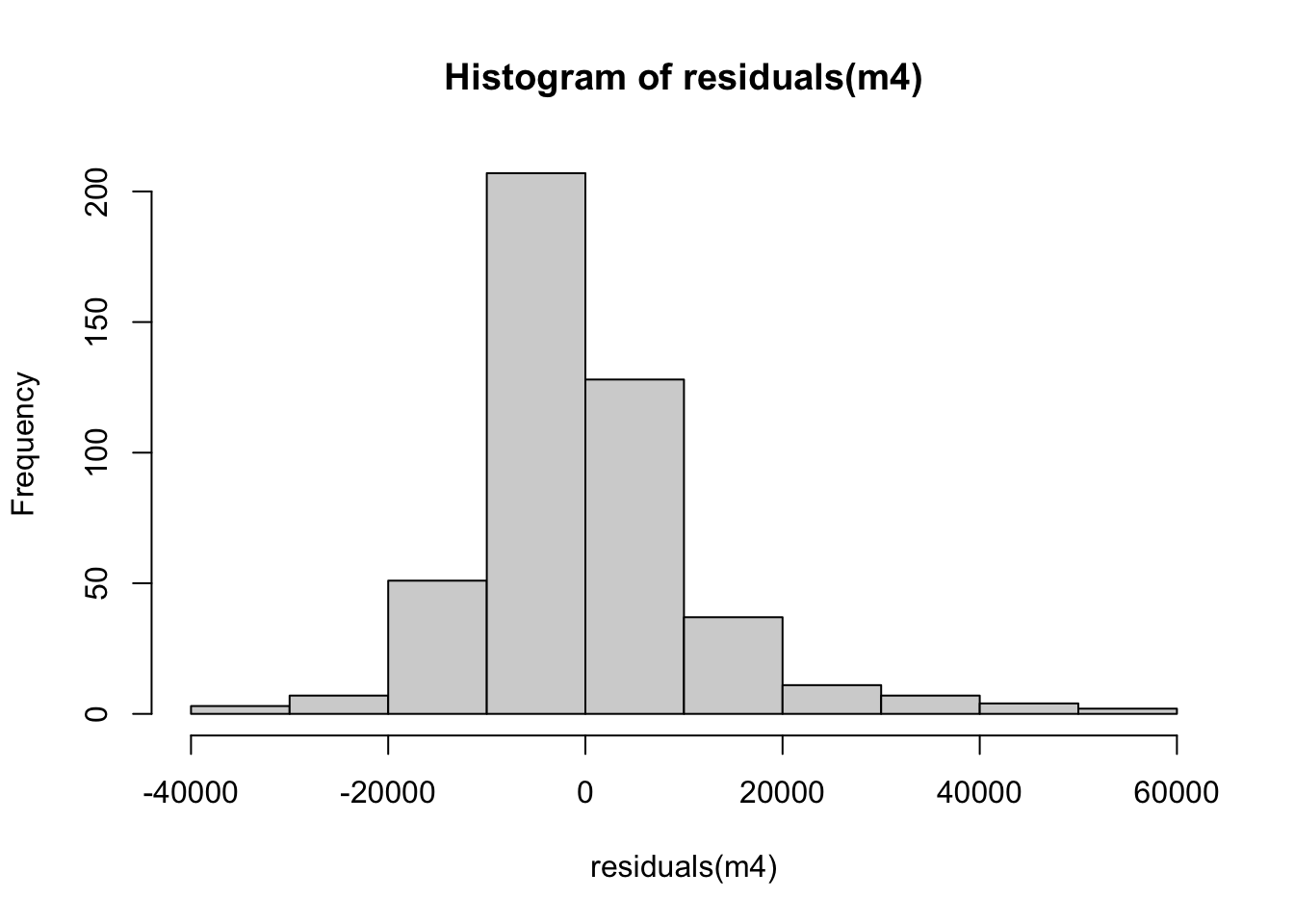
The distribution of the residuals in ‘m4’ looks overall normally distributed. However, the distribution is not perfectly symmetric. Therefore, we would advise conducting further checks to test the linear model assumptions.